Introduction
When comparing human and computer learning methods, one of the main differences is that humans learn from past experiences, or at least they try. Computers, on the other hand, are strict logic machines with zero common sense. If we want them to do something, then we have to give them detailed, step-by-step instructions on what that task is. This is why we write code and program computers, to follow those precise instructions. So, how is it that computers have the ability to learn? That’s where ‘Machine Learning’ comes into the picture.
Continue reading as we explore Machine Learning, discuss its lifecycle, and learn of its capabilities through open source frameworks in this article series.
What is Machine Learning?
Machine Learning is the branch of science that studies how computers can learn without being explicitly programmed. As the name implies, it provides the computer with the ability to learn. Serving as a helpful tool, Machine Learning can solve numerous practical problems, as user-cases are identified and Machine Learning algorithms are utilized to create a solution.
When we take a look at Machine Learning, its various applications in today’s world are vast, and are used in many more places than what would be expected in today’s world.
Applications of Machine Learning
Before we begin, let’s review some typical use cases where Machine Learning can be applied.
- Healthcare: Predicting patient diagnostics for doctors to review
- Social Network: Predicting specific match preferences on a dating website for better compatibility
- Finance: Predicting fraudulent activity on a credit card
- E-commerce: Predicting customer churn
- Biology: Finding patterns in gene mutations that could represent cancer
Machine Learning Lifecycle
Thinking of how Machine Learning can be applied across a wide range of industries, lets now focus on how the Machine Learning is managed; this is called Machine Learning Operations. This provides an end-to-end ML development process to design, build, and manage Machine Learning software that is testable while having the ability to be reproduced and developed over the course of time.
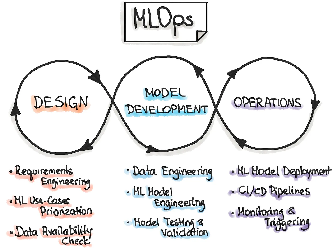
This process entails three different stages: the Design phase of the application, the Experimentation and Development phase, and the Operations phase.
In the first stage, the Design process is devoted to understanding the business and its related data to design the ML solution. First, we identify our potential user, design the Machine Learning solution to solve its problem, and assess the project’s further development. Primarily, we would act within two categories of problems — either increasing the user’s productivity or the interactivity of our application.
Furthermore, the design phase inspects the data needed to train the model while marking what the requirements are. These requirements are then taken and used to design the architecture and serving strategy of the application while creating a testing environment once the model is created.
The next phase, Experimentation and Development, aims to verify the applicability of machine learning for our problem by implementing Proof-of-Concept (PoC) for the model. Here, we run iteratively different steps that include identifying the suitable ML algorithm for our problem, data engineering, and model engineering. The main goal in this phase is to deliver a stable quality ML model to be produced.
Finally, the main focus of the Operations step is to deliver the previously developed ML model in production by using DevOps practices such as testing, versioning, continuous delivery, and monitoring.
All three phases are interconnected and influence each other. For example, the design decision will cultivate into the experimentation phase, ultimately affecting the deployment options during the final operations phase.
Problem to be solved
Now, lets take a look at a user case to provide an example. Many people struggle to get loans due to insufficient or non-existent credit histories.

Home Credit strives to broaden financial inclusion for the unbanked population by providing a positive and safe borrowing experience for the client. To ensure this underserved population has a favorable loan experience, Home Credit uses various alternative data — including telco and transactional information — to predict their clients’ repayment abilities.
While Home Credit is currently using multiple statistical and machine learning methods to make these predictions, they created a competition at Kaggle to help them unlock the full potential of their data.
Doing so will ensure that clients capable of repayment are not rejected and that loans are provided with a principal, maturity, and repayment calendar that will empower their clients to succeed.
Journey
Basically, all machine learning algorithms use some input data to create outputs. This input data is comprised of features, which are usually in the form of structured columns. Algorithms require features with some specific characteristics to work properly. This is where the need for feature engineering arises.
According to a survey in Forbes, data scientists spend almost 80% of their time on data preparation.
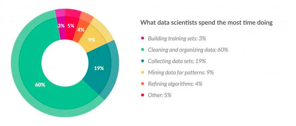
Feature engineering is the process of using domain knowledge of the data to create features that make machine learning algorithms work. If done correctly, feature engineering increases the predictive power of machine learning algorithms by creating features from raw data that help facilitate the machine learning process. Feature Engineering is an art.
We will aggregate and count values for home credit to incorporate information from:
- Application
- Previous application
- Positive cash balance
- Installments payments
- Bureau
- Bureau balance
- Credit card balance data filing into application files
Here are the definitions for each one and how they are inputted into the data system:
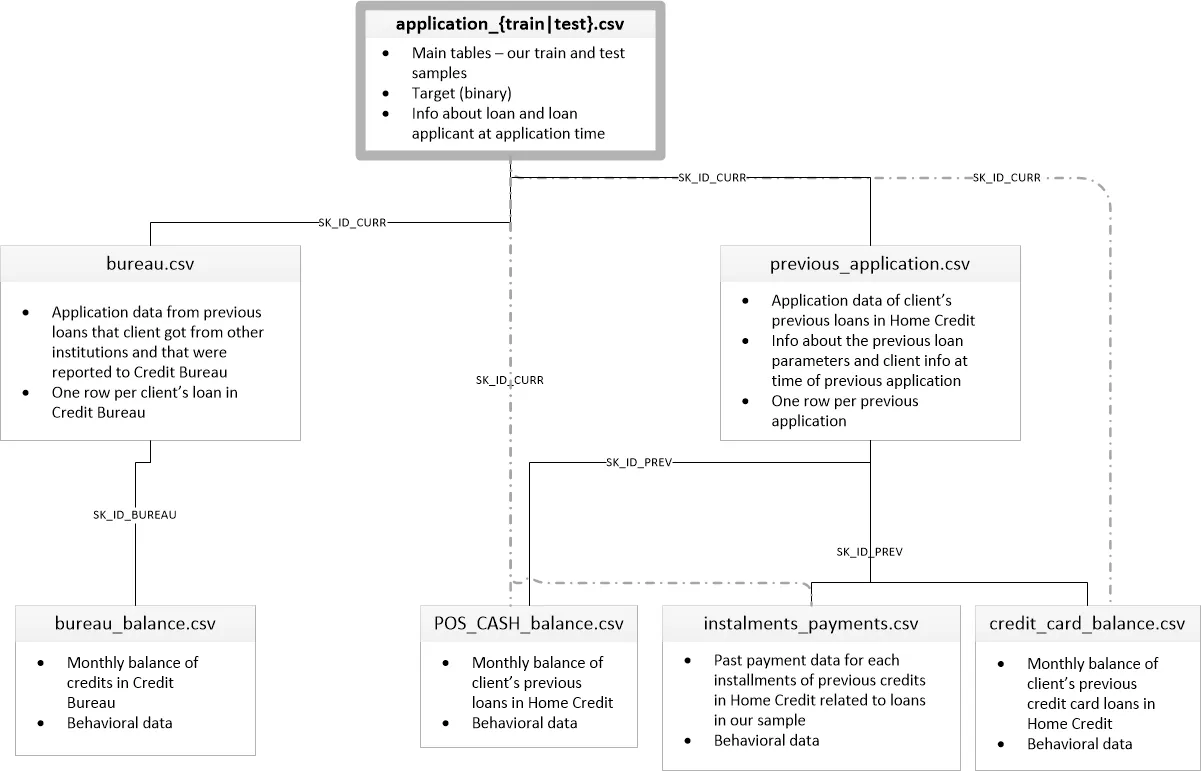
- Application: The main training and testing data with information about each loan application at Home Credit. Every loan has its row and is identified accordingly. The training application data comes with the TARGET indicating either 0: the loan was repaid, or 1: the loan was not repaid.
- Bureau: information about the client’s previous loans with other financial institutions reported to Home Credit. Each previous loan has its row.
- Bureau balance: monthly information about the previous loans. Each month has its row.
- Previous application (called previous): previous applications are for loans at Home Credit for clients who have loans in the application data. Each current loan in the application data can have multiple previous loans. Each previous application has one row and is identified by a feature titled SK_ID_PREV.
- Positive cash balance (called cash): monthly data about the previous point of sale or cash loans clients have had with Home Credit. Each row is one month of a previous point of sale or cash loan, and a single previous loan can have many rows.
- Credit card balance (called credit): monthly data about clients’ previous credit cards with Home Credit. Each row is one month of a credit card balance, and a single credit card can have many rows.
- Installments payment (called installments): payment history for previous loans at Home Credit. There is one row for every made payment and one row for every missed payment.
Here is a flow chart diagram of how this data is formatted into their system.
Manual Feature Engineering
Numerical Variables
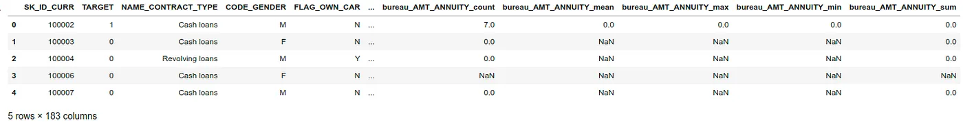
To illustrate the general process of manual feature engineering, we will first simply get the count of a client’s previous loans at other financial institutions.

Then we merge this information with the training data.
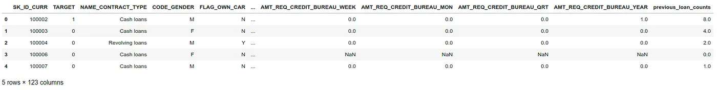
We can also aggregate numerical information using methods like mean, count, max, min, and sum functions.
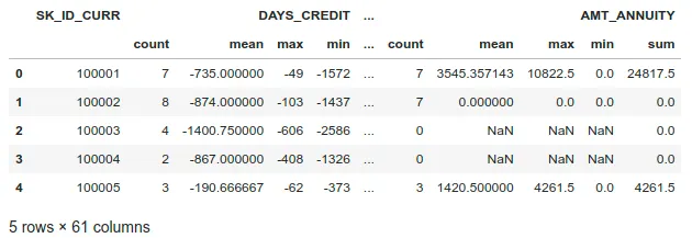
Once we create these new features, let’s merge them into the training set.
Categorical Variables
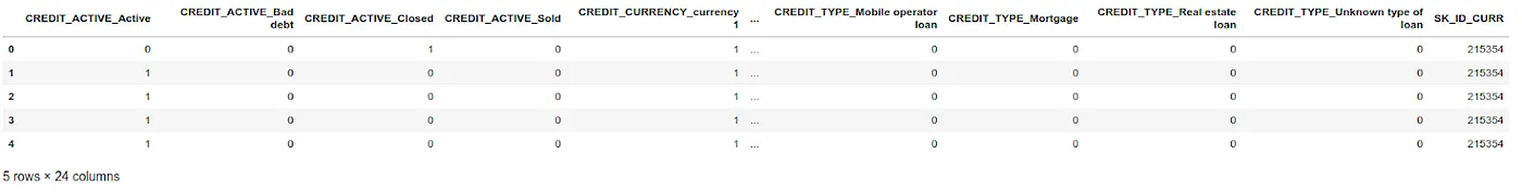
Now, we move from the numeric columns to the categorical columns. These are discrete string variables, so we cannot just calculate statistics such as mean and max (which only work with numeric variables).
Instead, we will rely on calculating value counts of each category within each categorical variable. Let’s do it for categorical features by doing one-hot encode bureau information with only the categorical columns (dtype == ‘object’).
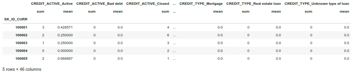
As we increase the number of tables we want to create new features for, we will need to code every step for every table. As you can imagine, this could be hard to maintain.
Automated Feature Engineering
Automated Feature Engineering (AutoFE) aims to help the data scientist with the problem of creating features by automatically building lots of new features from a dataset. Featuretools will not replace the data scientists themselves. Still, it will allow them to focus on more valuable parts of the machine learning pipeline, such as delivering robust models into production.
Next, we will touch on the concepts of AutoFE with featuretools and show how to implement it for the Home Credit Default Risk dataset.
To understand this framework, we need to understand its four main components:
- Entities and Entitysets
- Relationships
- Feature Primitives
- Deep Feature Synthesis
Entities and Entitysets
An Entity is simply a table. The observations are in the rows and the features are in the columns. An entity in Featuretools must have a unique index where none of the elements are duplicated.
Currently, only application, bureau, and previous have unique indices (SK_ID_CURR, SK_ID_BUREAU, and SK_ID_PREV, respectively). For the other dataframes, we need to pass in make_index=True and then specify the name of the index. Entities can also have time indices where each entry is identified by a unique time. (There are no date times in any data, but there are relative times, given in months or days, that we could consider treating as time variables).
An Entityset is a collection of tables and the relationships between them. It can be considered a data structure with its methods and attributes. Using an Entityset allows us to group multiple tables and manipulate them much quicker than individual tables.
Now, we define each entity or table of data. We need to pass in an index if the data has one or make_index=True if not.
Featuretools will automatically infer the types of variables, but we can also change them if needed. For example, if we have a categorical variable represented as an integer, we might want to let Featuretools know the right type.
Relationships
Relationships are a fundamental concept not only in Featuretools but in any relational database. The best way to think of a one-to-many relationship is with the parent-to-child analogy. A parent is a single individual but can have multiple children. The children can then have multiple children of their own. In a parent table, each individual has a single row. Each individual in the parent table can have multiple rows in the child table.
As an example, application has one row for each client (SK_ID_CURR) while the bureau has multiple previous loans (SK_ID_PREV) for each parent (SK_ID_CURR). Therefore, the bureau is the child of the application. The bureau in turn is the parent of bureau_balance because each loan has one row in bureau but multiple monthly records in bureau_balance.
Defining the relationships is relatively straightforward, and the competition diagram helps see the relationships. Now, we need to specify the parent and child variables for each relationship.
Altogether, there are a total of 6 relationships between the tables. Below we specify all six relationships and then add them to the Entityset.
Feature Primitives
Feature Primitives are operations applied to a table or a set of tables to create a new feature. These represent calculations, many of which we used in manual Feature Engineering, that can be stacked on top of each other to create complex features. Feature Primitives fall into two categories:
- Aggregation, a function that gathers child data points for each parent and then calculates a statistic such as max, min, mean or standard deviation. An example is calculating the maximum previous loan amount for each client. An aggregation works across multiple tables using relationships between tables. Examples:
- any: Test if any value is ‘True’.
- num_unique: Returns the number of unique categorical variables.
- last: Returns the last value.
- skew: Computes the skewness of a data set.
- trend: Calculates the slope of the linear trend of a variable over time.
- Transformation, an operation applied to one or more columns in a single table. An example would be taking the absolute value of a column, or finding the difference between two columns in one table. Examples:
- year: Transform a DateTime feature into the year.
- days_since: For each value of the base feature, compute the number of days between it
- absolute: Absolute value of the base feature.
- cum_min: Calculates the min of previous values of an instance for each value in a time-dependent entity.
- numeric_lag: Shifts an array of values by a specified number of periods.
Deep Feature Synthesis
Deep Feature Synthesis (DFS) is the process Featuretools uses to make new features. DFS stacks feature primitives to form features with a “depth” equal to the number of primitives. For example, if we take the maximum value of a client’s previous loans, that is a “deep feature” with a depth of 1. To create a feature with a depth of two, we could stack primitives by taking the maximum value of a client’s average monthly payments per previous loan. The original paper on AutoFE using DFS is worth a read.
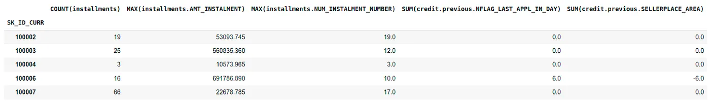
To perform DFS in Featuretools, we use the dfs function passing it into an entityset, the target_dataframe_name (where we want to create the features), the agg_primitives, the trans_primitives, and the max_depth of the features.
Here we will use the default aggregation and transformation primitives, a max depth of 2, and calculate primitives for the application entity.
To determine whether our basic implementation of Featuretools was useful, we can look at several results:
- Cross-validation scores using several different sets of features.
- Correlations: both between the features and the TARGET, and between features themselves
- Feature importance: determined by a machine learning model
Conclusion
In this article, we went through a basic implementation of using Automated Feature Engineering with Featuretools for the Home Credit Default Risk dataset. Moreover, Automated Feature Engineering took a fraction of the time spent on manual Feature Engineering while delivering comparable results.
Featuretools demonstrably adds value when included in a data scientist’s toolbox.
Here’s a Lightning Talk related to the topic of this article:
We think and we do!
Are you starting a new Machine Learning project and want to optimize the time of your Data Scientists by using Automated Feature Engineering and other MLOps techniques?
Contact us, we can help you!
Further reading and links
- Cover Photo by Clarisse Croset on Unsplash
- Example Repo
- Featuretools Documentation